Business Problem
Using the same data set from the Decision Tree Classification Blog from Week 1, the business problem is to predict which auto insurance customers are most likely to get in an automobile accident. The data set used to predict who will likely get in an accident contains 8,161 records of data with 15 variables representing various customer statistics. To predict the outcome, let’s review using a Clustering Methods.
Model
K-Means Clustering is one of the most common non-hierarchal clustering algorithms. The algorithm starts with identification of the number of clusters. It combs through the data and assigns it to a cluster based on the distance calculated between the data points. If the data point is closest to its own cluster it remains within that cluster. If the data point is not closest to its own cluster, it is assigned to the closest cluster nearby (Improved Outcomes, n.d.). This continues until all data points have been assigned a cluster. Generally, the analyst will run the algorithm several times to determine the appropriate number of clusters to get the best results.
Variables Used
The target variable is 0 for individuals who did not get in an accident and 1 for those who did get in an accident. The variables selected are marriage, time in force, claims ratio, claims frequency, motor vehicle points, city, age, income, years on job, gender, kids driving, cost per claim, high school or less education, license revoked and bluebook value. All clustering variables were standardized to have a mean of 0 and a standard deviation of 1.
Data were randomly split into a training set that included 70% of the observations (N=5713) and a test set that included 30% of the observations (N=2448). A series of k-means cluster analyses were conducted on the training data specifying k=1-9 clusters, using Euclidean distance. The variance in the clustering variables that was accounted for by the clusters (r-square) was plotted for each of the nine cluster solutions in an elbow curve to provide guidance for choosing the number of clusters to interpret.
Figure 1. Elbow curve of r-square values for the nine cluster solutions
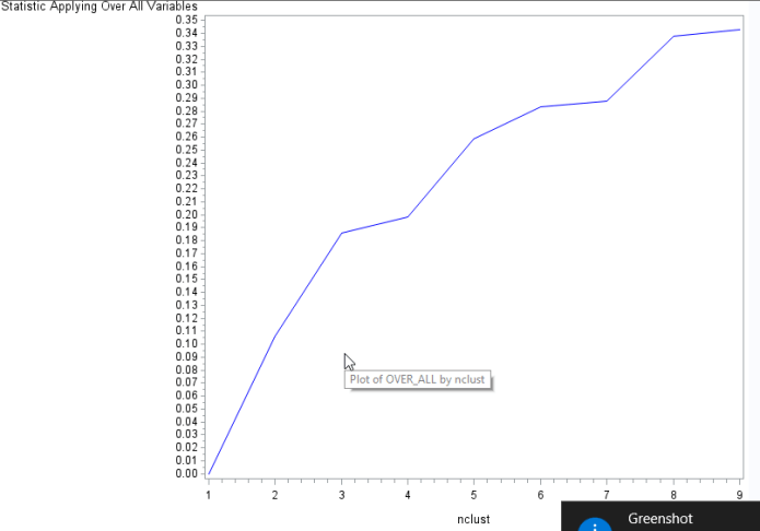

As we can see there is a break in cluster 3, 4, 5, 7 and 9. Review of the Eigenvalues shows in the the last column, the first five canonical variables account for about 99% of the total variation.

Review of the cluster means shows that cluster 3 has a higher probability of having their license revoked, higher claims with perhaps a lower income compared to cluster 1 and 2. Cluster 7 and 8 appear to demonstrate low level of claim activity with a higher income compared to the other clusters. Cluster 6 appears to group people that have low claim frequency, low motor vehicle points, are not young and don’t live in a city.
I chose to look at cluster 3, 5 and 7 to understand it’s content better since that made up 86% of the cumulative variation.
Cluster 3 on the left demonstrates a very large tightly populated cluster in the dark blue, with a scattered proportion separated from it. Then to the far left a tight nit bunch in the red, but that slightly overlaps with the blue cluster. Cluster 5 doesn’t add much separation but more of an overlap in the red cluster.


Cluster 7 shows a lot of overlap between cluster two and six as well as four and two. Its hard to determine the number of clusters based on this information alone.


The box plot shows that cluster four and six are individuals who will mostly likely not have an auto claim. This information is confirmed with cluster six when you review the means of each cluster variable within the cluster.
The tukey test shows that cluster 7 and 4 and cluster 7 and 6 differed from each other.

I’m not sold that cluster analysis is a great method for predicting auto claims. An individual can gain valuable insight about the populations, but it doesn’t appear to be a good method for predicting who will file an auto accident claim.
Code
%let PATH = C:\Users\mailb_000\Documents\Sas_data\nwu2016;
%let NAME = nwu;
%let LIB = &NAME..;
libname &NAME. “&PATH.”;
%let SCORE_ME = &LIB.LOGIT_INSURANCE_TEST;
%let INFILE = &LIB.LOGIT_INSURANCE;
%let SCRUBFILE = SCRUBFILE;
proc means data=&INFILE. mean median nmiss n p1 p99;
run;
data TEMPFILE;
set &INFILE;
R_EDUCATION = EDUCATION;
if R_EDUCATION = “z_High School” THEN R_EDUCATION = “High School”;
else if R_EDUCATION = “<High School” THEN R_EDUCATION = “High School”;
drop index;
drop education;
drop red_car;
drop target_amt;
run;
data &SCRUBFILE.;
SET TEMPFILE;
/*Fix missing values*/
IMP_AGE = AGE;
if missing (IMP_AGE) then IMP_AGE = 45;
IMP_INCOME = INCOME; /* Copy INCOME into IMP_INCOME*/
M_INCOME = 0;
if missing (IMP_INCOME) then do ;
if IMP_JOB = “Doctor” then do IMP_INCOME = 128680;end;
if IMP_JOB = “Lawyer” then do IMP_INCOME = 88304;end;
if IMP_JOB = “Manager” THEN do IMP_INCOME = 87461;end;
if IMP_JOB = “Professional” then do IMP_INCOME = 76593;end;
if IMP_JOB = “z_Blue Collar” then do IMP_INCOME = 58957; end;
if IMP_JOB = “Clerical” then do IMP_INCOME = 33861;end;
if IMP_JOB = “Home Maker” then do IMP_INCOME = 12073;end;
if IMP_JOB = “Student” then do IMP_INCOME = 6309;end;
M_INCOME = 1;
end;
IMP_YOJ = YOJ;
M_YOJ = 0;
if missing (IMP_YOJ) then do;
if IMP_JOB = “Student” then IMP_YOJ = 5;
else if IMP_JOB = “Home Maker” then IMP_YOJ = 4;
else IMP_YOJ =11;
M_YOJ = 1; end;
/*create dummy values*/
if urbanicity = ‘Highly Urban/ Urban’ then urbanicity = ‘1’;
else urbanicity = ‘0’;
CITY=urbanicity*1;
if PARENT1 = ‘Yes’ then parent1 = ‘1’;
else parent1 = ‘0’;
SINGLE_PARENT=parent1*1;
if sex = ‘M’ then sex = ‘1’;
else sex = ‘0’;
MALE=sex*1;
if revoked = ‘Yes’ then revoked = ‘1’;
else revoked = ‘0’;
LICENSE_REVOKED=revoked*1;
if mstatus = ‘Yes’ then mstatus = ‘1’;
else mstatus = ‘0’;
MARRIED=mstatus*1;
if car_use = ‘Commercial’ then car_use = ‘1’;
else car_use = ‘0’;
COMMERCIAL=car_use*1;
if KIDSDRIV > 0 then KIDSDRIV = ‘1’;
else KIDSDRIV = ‘0’;
KIDS_DRIVING = KIDSDRIV*1;
if R_EDUCATION = “High School” then HIGH_SCHOOL_OR_LESS = 1;
else HIGH_SCHOOL_OR_LESS = 0;
/*CAP – DEAL WITH OUTLIERS*/
CAP_BLUEBOOK = BLUEBOOK;
if CAP_BLUEBOOK >= 35000 THEN CAP_BLUEBOOK = 35000 /*95 percentile*/;
else if CAP_BLUEBOOK <= 5000 THEN CAP_BLUEBOOK = 5000 /*5 percentile*/;
/*New Variables*/
COST_PER_CLAIM = OLDCLAIM/CLM_FREQ ;
if missing (Cost_per_Claim) then Cost_per_Claim = 0;
CLAIM_RATIO_YIS = TIF/CLM_FREQ;
if missing (CLAIM_RATIO_YIS) then CLAIM_RATIO_YIS = 0;
run;
proc print data=&SCRUBFILE. (OBS=10); RUN;
data C2;
SET &SCRUBFILE.;
keep TARGET_FLAG;
keep SINGLE_PARENT;
keep LICENSE_REVOKED;
keep MARRIED;
keep COMMERCIAL;
keep KIDS_DRIVING;
keep HIGH_SCHOOL_OR_LESS;
keep MALE;
keep CITY;
keep CLM_FREQ;
keep MVR_PTS;
keep CLAIM_RATIO_YIS;
keep TIF;
keep IMP_YOJ;
keep IMP_AGE;
keep COST_PER_CLAIM;
keep OLDCLAIM;
keep CAP_BLUEBOOK;
keep IMP_INCOME;
run;
proc print data=C2 (obs=10); run;
data clust;
set C2;
* create a unique identifier to merge cluster assignment variable with
the main data set;
idnum=_n_;
keep idnum TARGET_FLAG TIF OLDCLAIM CLM_FREQ MVR_PTS IMP_AGE IMP_INCOME IMP_YOJ SINGLE_PARENT MALE LICENSE_REVOKED MARRIED CITY COMMERCIAL KIDS_DRIVING HIGH_SCHOOL_OR_LESS CAP_BLUEBOOK COST_PER_CLAIM CLAIM_RATIO_YIS ;
* delete observations with missing data;
if cmiss(of _all_) then delete;
run;
* Split data randomly into test and training data;
proc surveyselect data=clust out=traintest seed = 1234
samprate=0.7 method=srs outall;
run;
data clus_train;
set traintest;
if selected=1;
run;
data clus_test;
set traintest;
if selected=0;
run;
* standardize the clustering variables to have a mean of 0 and standard deviation of 1;
proc standard data=clus_train out=clustvar mean=0 std=1;
var TIF OLDCLAIM CLM_FREQ MVR_PTS IMP_AGE IMP_INCOME IMP_YOJ CITY SINGLE_PARENT MALE
LICENSE_REVOKED MARRIED COMMERCIAL KIDS_DRIVING HIGH_SCHOOL_OR_LESS CAP_BLUEBOOK COST_PER_CLAIM CLAIM_RATIO_YIS ;
run;
%macro kmean(K);
proc fastclus data=clustvar out=outdata&K. outstat=cluststat&K. maxclusters= &K. maxiter=300;
var TIF OLDCLAIM CLM_FREQ MVR_PTS IMP_AGE IMP_INCOME IMP_YOJ CITY SINGLE_PARENT MALE
LICENSE_REVOKED MARRIED COMMERCIAL KIDS_DRIVING HIGH_SCHOOL_OR_LESS CAP_BLUEBOOK COST_PER_CLAIM CLAIM_RATIO_YIS ;
run;
%mend;
%kmean(1);
%kmean(2);
%kmean(3);
%kmean(4);
%kmean(5);
%kmean(6);
%kmean(7);
%kmean(8);
%kmean(9);
* extract r-square values from each cluster solution and then merge them to plot elbow curve;
data clus1;
set cluststat1;
nclust=1;
if _type_=’RSQ’;
keep nclust over_all;
run;
data clus2;
set cluststat2;
nclust=2;
if _type_=’RSQ’;
keep nclust over_all;
run;
data clus3;
set cluststat3;
nclust=3;
if _type_=’RSQ’;
keep nclust over_all;
run;
data clus4;
set cluststat4;
nclust=4;
if _type_=’RSQ’;
keep nclust over_all;
run;
data clus5;
set cluststat5;
nclust=5;
if _type_=’RSQ’;
keep nclust over_all;
run;
data clus6;
set cluststat6;
nclust=6;
if _type_=’RSQ’;
keep nclust over_all;
run;
data clus7;
set cluststat7;
nclust=7;
if _type_=’RSQ’;
keep nclust over_all;
run;
data clus8;
set cluststat8;
nclust=8;
if _type_=’RSQ’;
keep nclust over_all;
run;
data clus9;
set cluststat9;
nclust=9;
if _type_=’RSQ’;
keep nclust over_all;
run;
data clusrsquare;
set clus1 clus2 clus3 clus4 clus5 clus6 clus7 clus8 clus9;
run;
* plot elbow curve using r-square values;
symbol1 color=blue interpol=join;
proc gplot data=clusrsquare;
plot over_all*nclust;
run;
*****************************************************************************************
further examine cluster solution for the number of clusters suggested by the elbow curve
*****************************************************************************************
* plot clusters for cluster solution;
proc candisc data=outdata5 out=clustcan;
class cluster;
var TIF OLDCLAIM CLM_FREQ MVR_PTS IMP_AGE IMP_INCOME IMP_YOJ CITY SINGLE_PARENT MALE
LICENSE_REVOKED MARRIED COMMERCIAL KIDS_DRIVING HIGH_SCHOOL_OR_LESS CAP_BLUEBOOK COST_PER_CLAIM CLAIM_RATIO_YIS ;
run;
proc sgplot data=clustcan;
scatter y=can2 x=can1 / group=cluster;
run;
* validate clusters on GPA;
* first merge clustering variable and assignment data with GPA data;
data gpa_data;
set clus_train;
keep idnum TARGET_FLAG;
run;
proc sort data=outdata7;
by idnum;
run;
proc sort data=gpa_data;
by idnum;
run;
data merged;
merge outdata7 gpa_data;
by idnum;
run;
proc sort data=merged;
by cluster;
run;
proc means data=merged;
var TARGET_FLAG;
by cluster;
run;
proc anova data=merged;
class cluster;
model TARGET_FLAG = cluster;
means cluster/tukey;
run;